

Creating a Stacked Bar Chart in Deneb with Vega-Lite

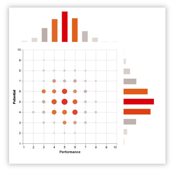
Welcome to this month’s Data Visualization Digest from DataAxe! Today, we’re diving into a powerful visualization tool: Deneb, a custom visual for Power BI that leverages Vega-Lite to create advanced charts. We’ll walk through a JSON specification to create a stacked bar chart, similar to the one shown below, which displays device types, their counts, and risk scores. By the end, you’ll understand each piece of the code, how to reproduce this chart, and how to adapt it for your data.
Let’s break down the JSON code step by step.
Step 1: Setting Up Deneb in Power BI
Before we dive into the code, ensure you have Deneb installed in Power BI:
Go to the Power BI visuals marketplace and search for "Deneb."
Add the Deneb visual to your report.
Drag the Deneb visual onto your canvas, and in the "Fields" pane, add your dataset. For this example, your dataset should have at least two fields: DeviceType (e.g., "Korbato Washer") and Sum of RiskScore (e.g., 1 to 10).
Now, click on the Deneb visual, go to the "Format" pane, and open the Deneb editor. This is where we’ll paste our JSON code.
Step 2: Understanding the JSON Structure
The JSON code we’re working with is a Vega-Lite specification. Vega-Lite is a high-level grammar for creating visualizations, and Deneb translates this into a chart within Power BI. Here’s the part of the JSON code we’ll dissect. I will provide the dataset on my Github at the end of the newsletter:
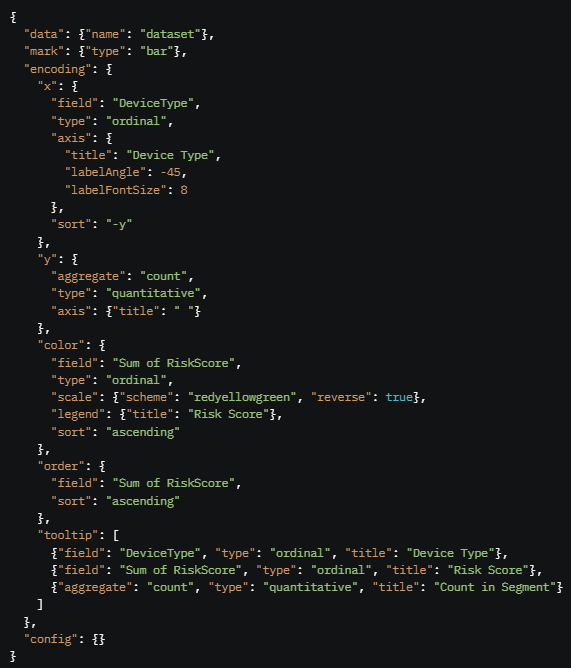
Let’s break this down into manageable sections.
Section 1: Data Binding

What it does: This line tells Vega-Lite where to get the data for the chart. In Deneb, "dataset" is a special name that refers to the data you’ve added to the Deneb visual in Power BI (via the "Fields" pane).
How to use it: Ensure your Power BI dataset has the fields DeviceType and Sum of RiskScore. Drag these fields into the Deneb visual’s "Values" section in Power BI. Deneb will automatically pass this data to Vega-Lite as "dataset".
Learning tip: If your dataset has a different structure, you might need to preprocess it in Power BI (e.g., using DAX) to match the expected fields.
Section 2: Defining the Mark

What it does: The mark property specifies the type of visualization. Here, "bar" creates a bar chart. Since we’re stacking bars (as seen in the image), Vega-Lite will handle the stacking automatically based on other encodings.
How to use it: This is straightforward—just set the type to "bar". If you wanted a different chart, you could change this to "line", "point", etc.
Learning tip: Vega-Lite’s documentation (https://vega.github.io/vega-lite/docs/mark.html) lists all available mark types. Experiment with different marks to see how they change your visualization.
Section 3: Encoding the X-Axis
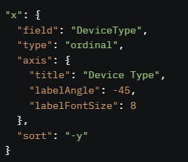
What it does: The x encoding defines the X-axis of the chart.
"field": "DeviceType": This tells Vega-Lite to use the DeviceType field from your dataset for the X-axis. Each unique device type (e.g., "Korbato Washer") becomes a bar.
"type": "ordinal": This specifies that DeviceType is a categorical field with no inherent numerical order (unlike, say, dates or numbers). Use "nominal" if the categories have no order at all, but "ordinal" works here since device types are distinct categories.
"axis": Customizes the X-axis appearance:
"title": "Device Type": Sets the axis title.
"labelAngle": -45: Rotates the labels (e.g., "Korbato Washer") by -45 degrees to prevent overlap, as seen in the image.
"labelFontSize": 8: Reduces the font size of the labels to fit them better.
"sort": "-y": Sorts the bars on the X-axis by the total height of each bar (the Y-axis value) in descending order. That’s why "Korbato Washer" (with the tallest bar) is on the left in the image.
How to use it: Replace "DeviceType" with the name of your categorical field. Adjust the axis properties (e.g., labelAngle, labelFontSize) to match your chart’s readability needs.
Learning tip: If your labels still overlap, try increasing the labelAngle (e.g., to -60) or reducing the labelFontSize further. You can also set "labelLimit" to truncate long labels.
Section 4: Encoding the Y-Axis

What it does: The y encoding defines the Y-axis.
"aggregate": "count": Instead of using a specific field, this counts the number of rows for each DeviceType and Sum of RiskScore combination. In the image, the Y-axis represents the count of devices (e.g., "Korbato Washer" has a total count of 13).
"type": "quantitative": Specifies that the Y-axis is numerical (since counts are numbers).
"axis": {"title": " "}: Sets the Y-axis title to a blank space. In the image, there’s no Y-axis title, which is why this is empty. You could set it to something like "Count of Devices" if desired.
How to use it: If your Y-axis should represent a different value (e.g., a sum of a field like Revenue), replace "aggregate": "count" with "aggregate": "sum" and add "field": "Revenue".
Learning tip: Vega-Lite supports various aggregations like "sum", "average", "min", "max", etc. Check the documentation (https://vega.github.io/vega-lite/docs/aggregate.html) to explore other options.
Section 5: Encoding the Color (Stacking by Risk Score)
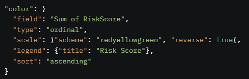
What it does: The color encoding creates the stacked segments within each bar, colored by the Sum of RiskScore field.
"field": "Sum of RiskScore": Uses the Sum of RiskScore field to determine the stack segments. In the image, each bar is split into segments for risk scores 1 to 10.
"type": "ordinal": Treats Sum of RiskScore as a categorical field (since risk scores are discrete values: 1, 2, 3, ..., 10). If Sum of RiskScore were a continuous number (e.g., 1.5, 2.7), you’d use "type": "quantitative" for a gradient.
"scale": {"scheme": "redyellowgreen", "reverse": true}: Defines the color scheme for the risk scores. The "redyellowgreen" scheme goes from red (high values) to yellow (middle) to green (low values). "reverse": true flips this, so low risk scores (e.g., 1) are green, and high scores (e.g., 10) are red, matching the image’s legend.
"legend": {"title": "Risk Score"}: Sets the title of the legend to "Risk Score," as seen in the image.
"sort": "ascending": Sorts the legend entries in ascending order (1 at the top, 10 at the bottom).
How to use it: Replace "Sum of RiskScore" with your stacking field. If your field is continuous, change "type" to "quantitative". You can explore other color schemes in Vega-Lite’s documentation (https://vega.github.io/vega-lite/docs/scale.html#scheme).
Learning tip: If the colors don’t match your expectations, try removing "reverse": true" or picking a different scheme (e.g., "blues", "viridis").
Section 6: Controlling the Stacking Order

What it does: The order encoding controls the stacking order within each bar.
"field": "Sum of RiskScore": Stacks the segments based on the Sum of RiskScore field.
"sort": "ascending": Stacks from lowest to highest risk score. In the image, risk score 1 (green) is at the bottom of each bar, and risk score 10 (red) is at the top.
How to use it: If you want high risk scores at the bottom, change "sort" to "descending".
Learning tip: The order encoding is crucial for stacked charts to ensure the visual hierarchy makes sense. Experiment with "sort" to see how it affects your chart.
Section 7: Adding Tooltips

What it does: The tooltip encoding defines what appears when you hover over a bar segment.
First entry: Shows the DeviceType (e.g., "Korbato Washer").
Second entry: Shows the Sum of RiskScore for that segment (e.g., 1, 2, ..., 10).
Third entry: Shows the count of devices in that specific segment (e.g., how many "Korbato Washer" devices have a risk score of 1).
How to use it: Add more fields to the tooltip array if you want to display additional information (e.g., {"field": "EquipmentId", "title": "Equipment ID"}).
Learning tip: Tooltips are a great way to make your chart interactive. Ensure the type matches your field (e.g., "quantitative" for numbers, "ordinal" or "nominal" for categories).
Section 8: Optional Configuration

What it does: The config section allows you to customize the overall appearance of the chart. In this example, it’s empty, but you could add properties like:
"view": {"stroke": "transparent"} to remove the border around the chart.
"bar": {"cornerRadius": 5} to add rounded corners to the bars.
How to use it: Add any Vega-Lite configuration options here to tweak the chart’s look and feel.
Learning tip: Check Vega-Lite’s configuration documentation (https://vega.github.io/vega-lite/docs/config.html) for more options.
Step 3: Putting It All Together
Copy the JSON code into the Deneb editor in Power BI.
Ensure your dataset has the fields DeviceType and Sum of RiskScore, and drag them into the Deneb visual’s "Values" section.
Click "Apply" in the Deneb editor. You should see a stacked bar chart like the one in the image, with device types on the X-axis, counts on the Y-axis, and stacks colored by risk score.
Step 4: Customizing for Your Data
Change the fields: Replace "DeviceType" and "Sum of RiskScore" with your own field names.
Adjust the color scheme: If "redyellowgreen" doesn’t suit your needs, try another scheme or define custom colors using "scale": {"range": ["#ff0000", "#00ff00"]}.
Modify the Y-axis: If you want to show a sum instead of a count, update the y encoding to "aggregate": "sum", "field": "YourField".
Tweak the appearance: Adjust labelAngle, labelFontSize, or add config options to match your style.
Key Takeaways
Data binding connects your Power BI dataset to Vega-Lite.
Encodings (x, y, color, etc.) define how your data is mapped to visual elements.
Customization (e.g., axis, scale, tooltip) makes your chart both functional and visually appealing.
Experimentation is key—try different mark types, color schemes, and aggregations to learn what works best for your data.
We hope this guide helps you create stunning visualizations with Deneb and Vega-Lite! If you have questions or want to share your creations, reply to this newsletter—we’d love to hear from you.
Here is the link to download the file. And a very special thank you to Greg Philps for troubleshooting with me.
The DataAxe Team